
Freezing Lake
Before you begin
You should know conduction through a slab, latent heat, conservation of mass and the density variation of water near \(4\,{}^\circ\mathrm{C}\). The early growth extension uses elementary integration.
Heat escapes through the ice, while the warmer lake bed supplies heat from below. The difference between these two heat flows determines whether the ice grows or melts. We will use this balance to find the initial growth rate and the final thickness.
The problem
At the instant considered, a large flat freshwater lake has a uniform ice sheet of thickness \(d_0=1.0\,\mathrm{cm}\) above liquid water of depth \(H_0=5.0\,\mathrm{m}\). A large cold reservoir holds the upper ice surface at \(T_s=-10\,{}^\circ\mathrm{C}\). A large warm reservoir holds the lake bed at \(T_b=4.0\,{}^\circ\mathrm{C}\). The ice–water interface is at \(T_m=0\,{}^\circ\mathrm{C}\).
| Property | Liquid water | Ice |
|---|---|---|
| Conductivity \(\kappa\) | \(0.57\,\mathrm{W\,m^{-1}\,K^{-1}}\) | \(2.2\,\mathrm{W\,m^{-1}\,K^{-1}}\) |
| Density \(\rho\) | \(999\,\mathrm{kg\,m^{-3}}\) | \(920\,\mathrm{kg\,m^{-3}}\) |
| Specific heat capacity \(c\) | \(4200\,\mathrm{J\,kg^{-1}\,K^{-1}}\) | \(2100\,\mathrm{J\,kg^{-1}\,K^{-1}}\) |
The latent heat of fusion is \(L_f=3.30\times10^5\,\mathrm{J\,kg^{-1}}\). For a slab, conduction power is \(P=\kappa A\Delta T/\ell\), where \(A\) is its face area and \(\ell\) is its thickness.
Assume vertical heat flow and use the quasi-steady approximation: each layer has a linear temperature profile at the instant considered. In the leading energy balance, retain latent heat but neglect changing sensible heat stored in the layers and work against gravity. Neglect evaporation, sublimation and sideways heat flow.
The horizontal area and total mass of water plus ice remain fixed. The ice surface may rise as freezing proceeds. Ignore water convection, then justify this in part c.
Part a. Find the initial rate of increase of the ice thickness.
Part b. Find the final ice thickness if both boundary temperatures are maintained for a long time.
Part c. Explain why buoyancy-driven convection can be neglected in the water.
Part a Initial growth of the ice
Identify both heat fluxes
Let \(d\) be the current ice thickness and \(H\) the remaining water depth. Take upward heat flux as positive. Heat leaves the interface through the ice, but heat also reaches it through the warmer water below.
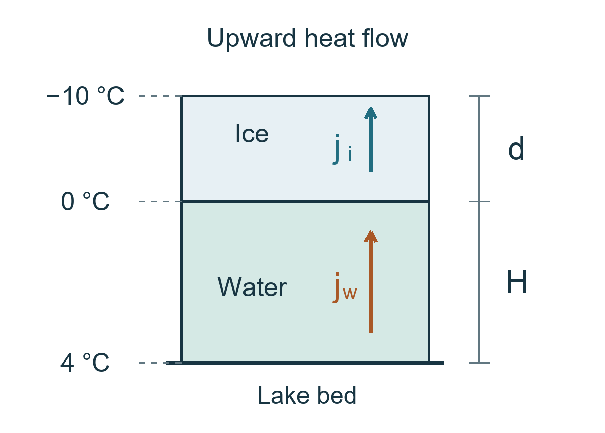
The temperature differences across the ice and water are \(\Delta T_{\mathrm{i}}=10\,\mathrm{K}\) and \(\Delta T_{\mathrm{w}}=4.0\,\mathrm{K}\). Conduction gives
At the stated initial thicknesses,
Use the difference to find the freezing rate
If the ice thickens by \(\mathrm{d}d\) over area \(A\), the newly formed ice has mass \(\rho_{\mathrm{i}}A\,\mathrm{d}d\). Freezing releases latent heat \(\rho_{\mathrm{i}}AL_f\,\mathrm{d}d\). The interface energy balance is
Therefore,
At the initial instant,
The initial growth rate is approximately \(2.6\,\mathrm{cm\,h^{-1}}\).
The water supplies only about \(0.021\%\) of the initial ice flux, so omitting it changes little here. We must still identify this incoming heat; it becomes essential in part b.
Which density should we use? The question asks for the thickness of newly formed ice, so use \(\rho_{\mathrm{i}}\). The downward speed of the interface is \(\mu\,\mathrm{d}d/\mathrm{d}t\), where \(\mu=\rho_{\mathrm{i}}/\rho_{\mathrm{w}}\). This is smaller than the growth rate of ice thickness because the upper surface also rises.
Part b The final ice thickness
Conserve mass rather than total depth
The density ratio is \(\mu=920/999\). Conservation of mass per unit horizontal area gives
Hence
where
The quantity \(D\) is the depth that the conserved mass would occupy if it were all liquid. It is not the physical depth \(H+d\). Ice is less dense than water, so the physical depth increases as freezing proceeds.
Make the interface stationary
At the final thickness, heat arriving at the interface equals heat leaving it:
Thus
Combine this with the mass balance to obtain
Numerically,
The final ice thickness is approximately \(4.89\,\mathrm{m}\). The remaining liquid depth and the common heat flux are
About half a metre of liquid remains. The lake does not freeze completely in this ideal model because the bed continues to supply heat.
Check the expansion and the continuing heat flow
The total final depth is \(d_{\mathrm{eq}}+H_{\mathrm{eq}}=5.3958\,\mathrm{m}\), compared with \(5.0100\,\mathrm{m}\) initially. The upper surface rises by approximately \(0.386\,\mathrm{m}\). Imposing a constant total depth would incorrectly prevent this expansion.
Although the interface is stationary, heat still flows upward at \(4.50\,\mathrm{W\,m^{-2}}\). This is a steady state with heat transfer, not thermal equilibrium at one temperature.
Part c Stable water layers
Why warmer water stays below colder water
Fresh water has its greatest density close to \(4\,{}^\circ\mathrm{C}\). Between \(0\,{}^\circ\mathrm{C}\) and \(4\,{}^\circ\mathrm{C}\), warming increases its density.
Here, water near the ice is at \(0\,{}^\circ\mathrm{C}\) and water at the bed is at \(4\,{}^\circ\mathrm{C}\). Denser water is already below less dense water. Exchanging two layers would put denser water higher and increase gravitational potential energy. This is a stable arrangement.
The temperature difference therefore does not drive the overturning convection familiar in water above \(4\,{}^\circ\mathrm{C}\) heated from below. In the stated model, heat passes through the water by conduction. The constant density used in the mass calculation is a numerical approximation; the qualitative density variation determines stability.
Why the final ice thickness is also stable
This is a separate argument about freezing and melting. Conservation of mass fixes \(H=D-\mu d\), so
As the ice thickens, its conduction path becomes longer and \(j_{\mathrm{i}}\) decreases. The remaining water becomes shallower and \(j_{\mathrm{w}}\) increases.
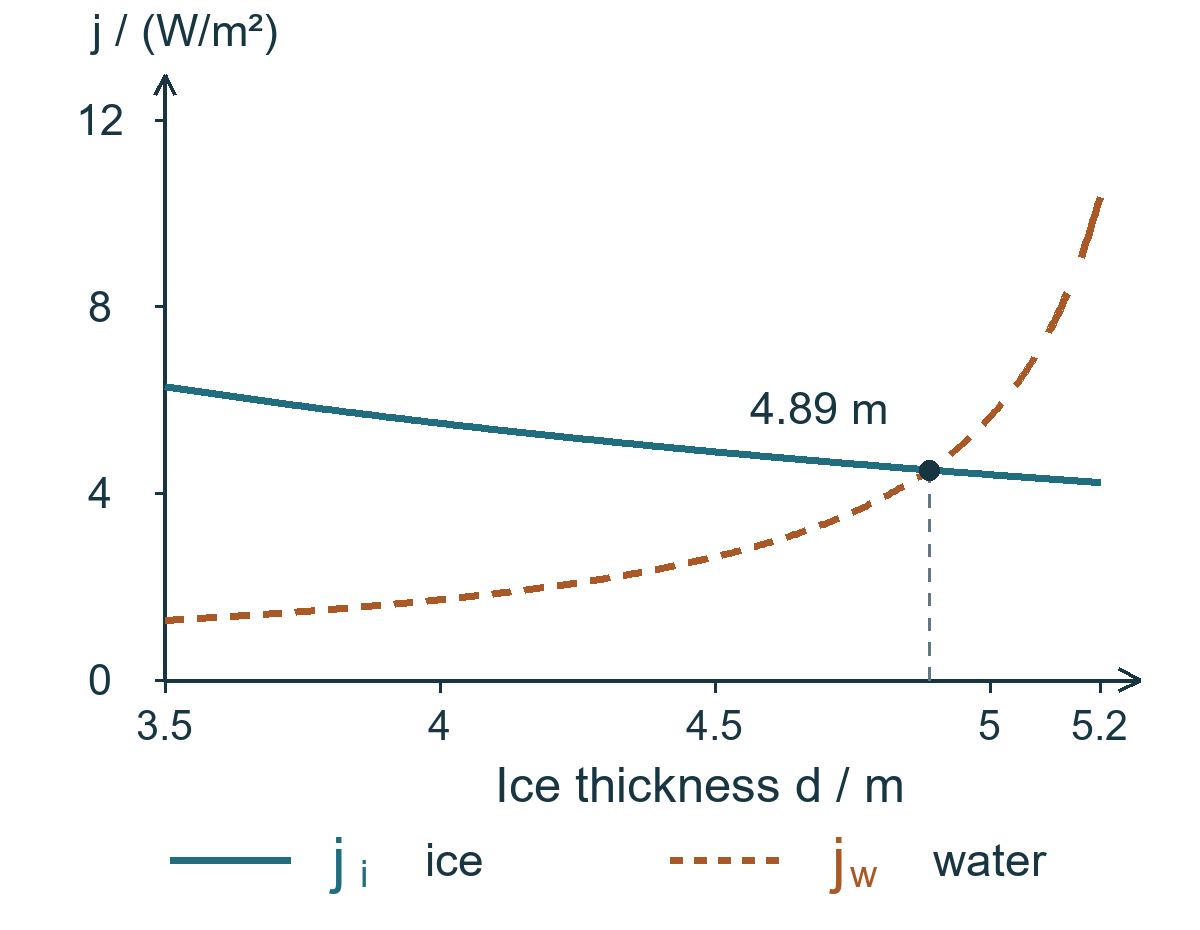
If the ice is slightly thinner than its final thickness, \(j_{\mathrm{i}}>j_{\mathrm{w}}\) and excess heat removal causes further freezing. If it is slightly thicker, \(j_{\mathrm{i}}<j_{\mathrm{w}}\) and excess incoming heat causes melting. Both changes move the thickness back toward \(d_{\mathrm{eq}}\).
Keep the two balances distinct. Equal heat fluxes describe the stationary interface in part b. During freezing, their difference accounts for latent heat released per unit area per second:
Extension How the freezing rate changes
The early growth law
While the water flux is much smaller than the ice flux, the leading balance becomes
Multiply by \(d\) and integrate from the initial thickness:
Therefore,
Once the increase in squared thickness is much larger than \(d_0^2\), thickness grows approximately as \(\sqrt{t}\) rather than as \(t\). The increasing conduction path slows the heat loss.
For growth from \(1.0\,\mathrm{cm}\) to \(2.0\,\mathrm{cm}\), the same leading model gives
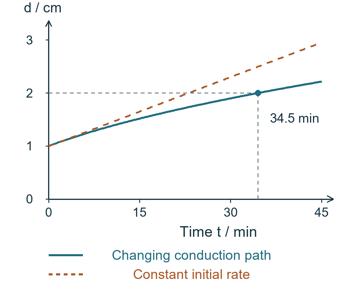
Using the initial rate as a constant would give only about \(23\,\mathrm{min}\). The square-root estimate accounts for the changing conduction path. Do not extrapolate it to the final thickness, where the water heat flux is no longer negligible.
What the approximation includes
The main answers use the prescribed quasi-steady, latent-heat model. The “initial” rate refers to the stated layer thicknesses with linear temperature profiles already assumed. It is not the instantaneous response to a sudden change in surface temperature.
The supplied specific heat capacities matter in a more detailed transient treatment because temperatures within both layers change as the interface moves. They do not enter the leading calculation here. Adding an isolated sensible-heat term to the latent heat does not give an exact transient solution: the temperature profiles and heat fluxes must also be refined.
Points to remember
Subtract heat arriving through the water from heat leaving through the ice.
Convert freezing mass to ice thickness using the ice density.
Conserve total mass and allow the physical depth to increase.
At the final thickness, freezing stops but heat flow continues.
Distinguish stability of the water layers from stability of the ice thickness.
Sources and further reading
The source problem is USAPhO 2016, Part A, Question A4. See the AAPT question paper, PDF page 6, and official solutions, PDF pages 11 to 13.
All three original tasks and numerical data are retained in fresh wording, with the leading approximation stated explicitly. The selected handout’s expansion check, flux comparison and early growth calculation are also retained. All three scientific figures are independently prepared. The early growth plot compares that calculation with a constant initial rate.