
Radiation and the Greenhouse Effect
Before you begin
You should know the Stefan–Boltzmann law, energy conservation, geometric series and elementary differentiation. This article covers the solar-constant calculation in A1 and all six tasks B1 to B6 of one connected Olympiad problem.
How do sunlight reflections and infrared absorption determine the temperatures of a surface and its atmosphere? We will build the energy balances step by step, then calculate how both equilibrium temperatures respond to a small change in atmospheric emissivity.
The model
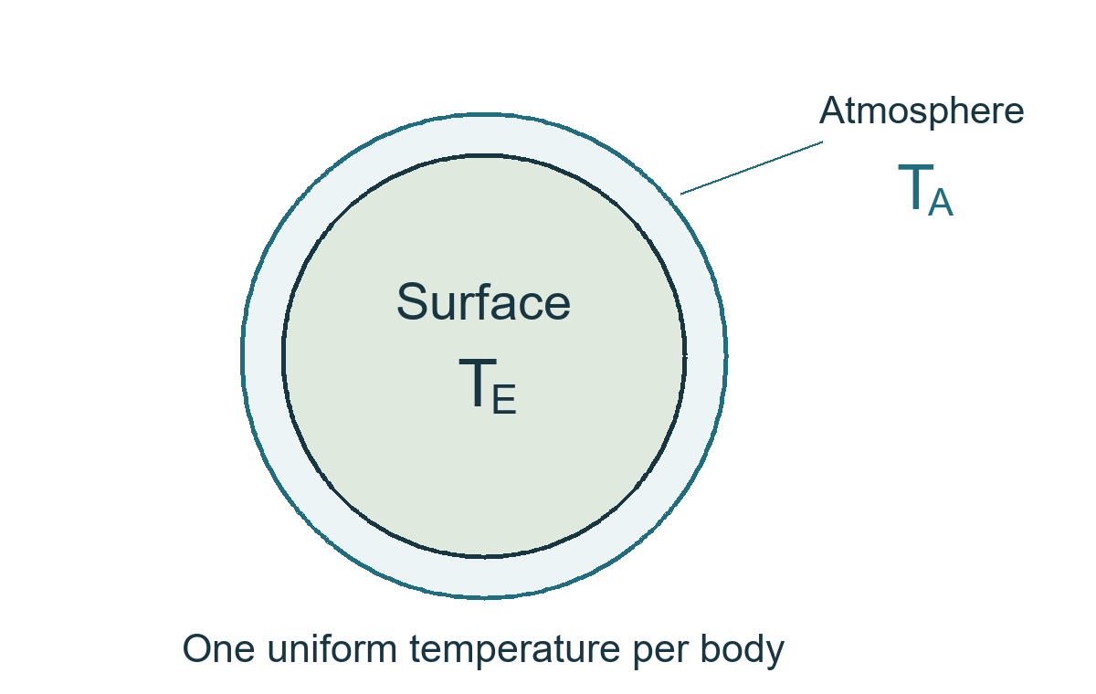
Treat Earth as a sphere with a uniform surface temperature \(T_{E}\), covered by a thin, isothermal atmospheric layer at \(T_{A}\). Each face of the layer has effectively the same area as the Earth’s surface. All states considered are steady equilibria.
Use two idealized radiation bands: all incoming sunlight is shortwave, and all thermal emission from Earth and its atmosphere is longwave infrared. Their optical properties are:
| Radiation band | Atmosphere | Earth surface |
|---|---|---|
| Shortwave sunlight | Reflects \(r_A\) from either side; absorbs zero; transmits \(1-r_A\). | Reflects \(r_E\) and absorbs \(1-r_E\). |
| Longwave infrared | Absorbs \(\varepsilon\); reflects zero; transmits \(1-\varepsilon\). Each face emits \(\varepsilon\sigma T_A^4\). | Absorbs all infrared; emits \(\sigma T_E^4\). |
Incoming infrared radiation from space is neglected. Unless a task explicitly introduces nonradiative transfer, radiation is the only heat-transfer mechanism. All temperatures must be in kelvin.
Notation that matters. The combined albedo \(\alpha\) is the fraction of incident solar power that eventually returns to space. It includes all repeated reflections; it is distinct from \(r_{A}\), \(r_{E}\) and the infrared emissivity \(\varepsilon\).
Data and questions
The Sun is a spherical blackbody. Use the following data and retain unrounded intermediate values.
| Quantity | Symbol | Value |
|---|---|---|
| Stefan–Boltzmann constant | \(\sigma\) | \(5.67\times10^{-8}\,\mathrm{W\,m^{-2}\,K^{-4}}\) |
| Solar surface temperature | \(T_S\) | \(5770\,\mathrm{K}\) |
| Solar radius | \(R_S\) | \(6.96\times10^8\,\mathrm{m}\) |
| Sun–Earth centre-to-centre distance | \(d\) | \(1.50\times10^{11}\,\mathrm{m}\) |
| Atmospheric shortwave reflectivity | \(r_A\) | \(0.255\) |
| Surface shortwave reflectivity from B2 | \(r_E\) | \(0.102\) |
Preparation (A1). Find the solar constant \(S_{0}\): solar power per unit area perpendicular to the rays at Earth’s orbit. Explain why the mean incident flux over the entire Earth is \(S_{0}/4\).
B1 · An opaque infrared atmosphere. Set \(r_{E}=0\) and \(\varepsilon=1\), with no nonradiative transfer. Determine the equilibrium temperatures \(T_{E}\) and \(T_{A}\).
B2 · Repeated shortwave reflections. Restore \(r_{E}=0.102\) for this and all subsequent parts. Derive the combined albedo \(\alpha\) in terms of \(r_{A}\) and \(r_{E}\), including every reflection. Evaluate it numerically.
B3 · Partial infrared absorption. With no nonradiative transfer, derive \(T_{E}\) in terms of \(\sigma\), \(\alpha\), \(S_{0}\) and \(\varepsilon\). What atmospheric emissivity gives \(T_{E}=288\ \mathrm{K}\)?
B4 · Small change in emissivity. For the B3 model, derive \(dT_{E}/d\varepsilon\). Estimate the surface warming when emissivity increases by 1% relative to its B3 value, holding \(\alpha\) and \(S_{0}\) fixed. Thus \(\Delta\varepsilon=0.01\varepsilon\); use a first-order approximation.
B5 · Add nonradiative transfer. Now allow an upward heat flux per unit Earth surface area of \(J=k\left( T_{E}-T_{A} \right)\), where \(k\) is constant. Make a new calibration using \(T_{E}=288\ \mathrm{K}\) and \(T_{A}=245\ \mathrm{K}\). Determine both \(\varepsilon\) and \(k\).
B6 · Coupled temperature response. Keep the B5 value of \(k\), the albedo and the solar constant fixed. Differentiate the two heat-balance equations to obtain simultaneous linear equations for \(dT_{E}/d\varepsilon\) and \(dT_{A}/d\varepsilon\). Estimate the first-order surface warming for a 1% relative increase from the B5 emissivity.
Solar input and B1
Find the solar constant
The Sun’s luminosity is its emitting area multiplied by its blackbody flux. At distance \(d\), this power is spread over a sphere of area \(4\pi d^{2}\):
Substitution gives \(S_{0}=1353.0763\ \mathrm{W}\,\mathrm{m}^{-2}\). This is the incident flux on a plane perpendicular to the rays, not the mean over the globe.
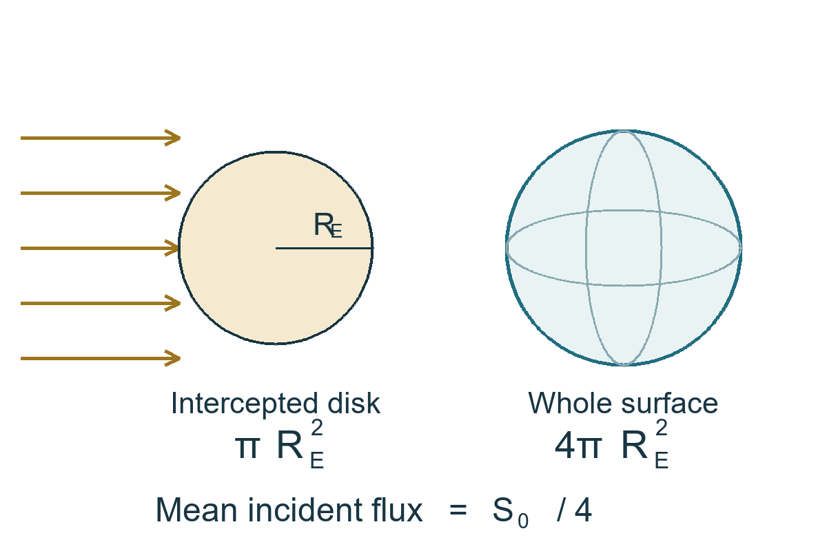
Let \(F\) denote absorbed solar power per unit area of the entire Earth surface. The Earth intercepts sunlight over \(\pi R_{E}^{2}\), so
Balance the two bodies separately
In B1 the surface reflects no sunlight, so \(\alpha=r_{A}\). Hence \(F_1=(1-r_A)S_0/4\), giving \(252.0105\,\mathrm{W\,m^{-2}}\). The surface receives both sunlight and downward infrared; the atmosphere absorbs all surface infrared and radiates from two faces:
Therefore \(F_{1}=\sigma T_{A}^{4}\), giving
Energy check. Only the atmosphere radiates to space in B1. Its upward flux is \(\sigma T_{A}^{4}=F_{1}\), exactly the absorbed solar flux. The downward atmospheric flux is an internal exchange, not an additional external energy source.
B2 Count the shortwave reflections
Follow one unit of shortwave solar power incident on the atmosphere. A fraction \(r_{A}\) returns immediately to space. The remaining fraction, \(1-r_{A}\), reaches the surface.
Count the escaping contributions
A ray reflected by the surface must pass through the atmosphere again to escape. Its first escaping contribution therefore contains two transmission factors:
If the ray does not escape on that return, atmospheric reflection sends it downward and surface reflection sends it upward again. Every extra round trip contributes a factor \(r_{A}r_{E}\).
| Escape route | Fraction of original incident power |
|---|---|
| Direct atmospheric reflection | \(r_A\) |
| First surface return | \((1-r_A)^2r_E\) |
| One additional round trip | \((1-r_A)^2r_E(r_A r_E)\) |
| \(n\) additional round trips | \((1-r_A)^2r_E(r_A r_E)^n\) |
Adding the direct reflection and the convergent geometric series gives
Here \(r_{A}r_{E}=0.02601\), so
Check by counting absorbed sunlight
On its first arrival, the surface absorbs \(\left( 1-r_{A} \right)\left( 1-r_{E} \right)\) of the original power. Every later arrival is smaller by the same factor \(r_{A}r_{E}\). Thus
This verifies that reflected and absorbed fractions add to one. Since the atmosphere absorbs no shortwave radiation in this model, all of \(F\) is deposited at the surface.
Useful limiting cases. If \(r_{E}=0\), then \(\alpha=r_{A}\), as in B1. If \(r_{A}=0\), then \(\alpha=r_{E}\). These checks catch an incorrect transmission factor or a missing direct reflection.
B3 and B4 Radiation only
B3 Determine the emissivity
Retain \(F=232.3488\ \mathrm{W}\,\mathrm{m}^{-2}\). The surface remains a blackbody in infrared, but the atmosphere now absorbs only the fraction \(\varepsilon\) of the surface emission:
For \(\varepsilon>0\), the second equation gives \(T_{A}^{4}=T_{E}^{4}/2\). Inserting this into the surface balance yields
At \(T_{E}=288\ \mathrm{K}\), the surface emission is \(\sigma T_{E}^{4}=390.0794\ \mathrm{W}\,\mathrm{m}^{-2}\). Therefore
The corresponding atmospheric temperature is \(T_{A}=(288\,\mathrm{K})/2^{1/4}=242.1782\,\mathrm{K}\).
B4 Differentiate before substituting
Hold \(F\) fixed. Taking logarithms of the expression for \(T_{E}\) gives
Evaluate at the B3 equilibrium: \(dT_{E}/d\varepsilon=60.4387\ \mathrm{K}\) per unit change in emissivity. A relative increase of 1% means
Physical interpretation. Higher infrared emissivity increases the atmosphere’s absorption and its downward emission. The new equilibrium needs a higher surface temperature to restore the outgoing energy flux. The positive derivative expresses this response within the stated model.
Boundary check. As \(\varepsilon\to 0\), the surface tends to \((F/\sigma)^{1/4}\), or \(253.0\,\mathrm{K}\). At exactly \(\varepsilon=0\), a purely radiative atmosphere neither absorbs nor emits; its temperature is undetermined. Do not divide its balance by zero.
B5 Add nonradiative transfer
Adding \(J=k\left( T_{E}-T_{A} \right)\) changes both balances. We must recalibrate the emissivity using the new pair \(T_{E}=288\ \mathrm{K}\), \(T_{A}=245\ \mathrm{K}\); the B3 value is no longer the required one.
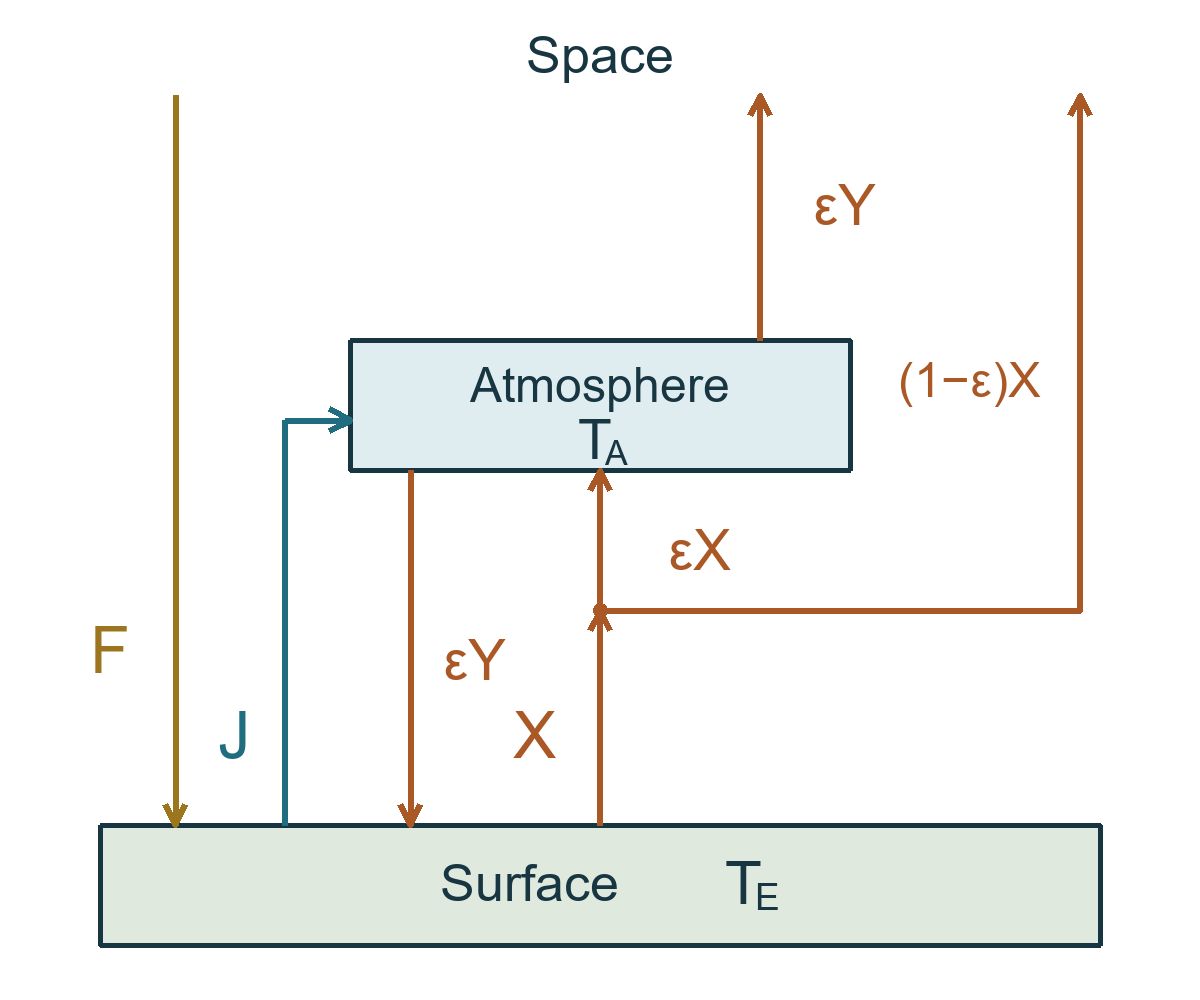
For compact notation, put \(X=\sigma T_{E}^{4}\) and \(Y=\sigma T_{A}^{4}\). The atmosphere emits \(\varepsilon Y\) from each face. All fluxes below are per unit area of the entire Earth surface.
Use the external energy balance for emissivity
The two local balances are
Adding them cancels \(J\) and the internal radiation exchange:
At the specified temperatures, \(X=390.0794\) and \(Y=204.2901\), both in \(\mathrm{W}\,\mathrm{m}^{-2}\). Hence
Recover the nonradiative coefficient
The atmospheric balance gives \(J=\varepsilon\left( 2Y-X \right)=15.7068\ \mathrm{W}\,\mathrm{m}^{-2}\). Since \(T_{E}-T_{A}=43\ \mathrm{K}\),
Here \(k\) is a heat-transfer coefficient, with units of flux divided by temperature difference. Its positive value is consistent with upward transfer from the warmer surface. The outgoing infrared flux, \(\left( 1-\varepsilon \right)X+\varepsilon Y\), is \(232.3488\ \mathrm{W}\,\mathrm{m}^{-2}\), equal to \(F\).
B6 Allow both temperatures to change
Set \(x=dT_{E}/d\varepsilon\) and \(y=dT_{A}/d\varepsilon\). In this part \(F\) and the B5 coefficient \(k\) are fixed; both temperatures are allowed to change with emissivity.
Apply the product rule to both balances
For example, differentiating the downward atmospheric radiation gives
Also, \(dJ/d\varepsilon=k\left( x-y \right)\), because a constant coefficient does not imply a constant heat flux. Differentiating \(F+\varepsilon\sigma T_{A}^{4}=\sigma T_{E}^{4}+k\left( T_{E}-T_{A} \right)\) gives
Differentiating \(\varepsilon\sigma T_{E}^{4}+k\left( T_{E}-T_{A} \right)=2\varepsilon\sigma T_{A}^{4}\) gives
Solve the two linear equations
Substitute the B5 equilibrium values, retaining extra digits in the coefficients. In the following two equations, the coefficients are in watts per square metre per kelvin, and the right-hand sides are in watts per square metre:
The coefficients have units \(\mathrm{W}\,\mathrm{m}^{-2}\,\mathrm{K}^{-1}\) and the right-hand sides have units \(\mathrm{W}\,\mathrm{m}^{-2}\). Multiply the first equation by \(6.028537\) and the second by \(3.196906\), then subtract to eliminate \(y\). Back-substitution gives the two temperature derivatives, in kelvin per unit change in emissivity:
Use the B5 emissivity for the 1% change
An additional result is \(\Delta T_{A}\simeq y\Delta\varepsilon=0.405585\ \mathrm{K}\). The surface warms more than the atmosphere, so the temperature difference and \(J\) both increase slightly even though \(k\) stays fixed.
Why this part is demanding. Emissivity multiplies a temperature-dependent radiation term, while the nonradiative flux depends on both temperatures. Omitting either product-rule term, or holding \(T_{A}\) fixed, changes the answer.
The temperatures and responses describe the specified one-layer equilibrium model. They are not a direct forecast of Earth’s climate. Extra intermediate digits are shown for checking; the summary uses three significant figures.
Answers and checks
| Part | Result |
|---|---|
| A1 | \(S_0=1.35\times10^3\,\mathrm{W\,m^{-2}}\); mean incident flux \(S_0/4\). |
| B1 | \(T_E=307\,\mathrm{K}\) and \(T_A=258\,\mathrm{K}\). |
| B2 | \(\alpha=0.313\) and \(F=232\,\mathrm{W\,m^{-2}}\). |
| B3 | \(\varepsilon_{\mathrm{rad}}=0.809\). |
| B4 | First-order surface warming \(\Delta T_E=0.489\,\mathrm{K}\). |
| B5 | \(\varepsilon_{\mathrm{coupled}}=0.849\) and \(k=0.365\,\mathrm{W\,m^{-2}\,K^{-1}}\). |
| B6 | First-order surface warming \(\Delta T_E=0.524\,\mathrm{K}\). |
Check the small-change approximation
The question requests derivative estimates. As an independent check, the equilibrium equations can also be solved with \(\varepsilon_{\mathrm{new}}=1.01\varepsilon_{\mathrm{old}}\) without linearization:
| Model | First-order \(\Delta T_E\) | Exact finite-change \(\Delta T_E\) |
|---|---|---|
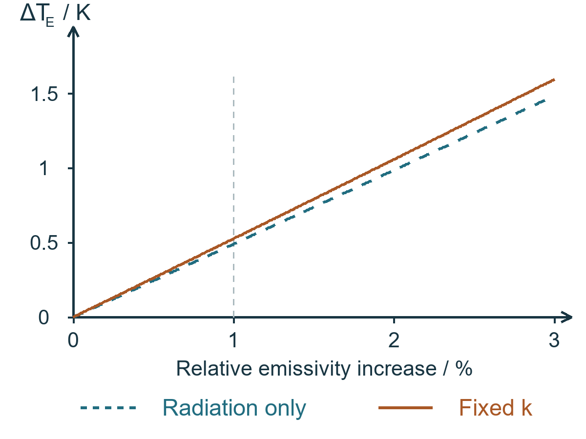
| Radiation only in B4 | \(0.488774\,\mathrm{K}\) | \(0.490858\,\mathrm{K}\) |
| Fixed \(k\) in B6 | \(0.524117\,\mathrm{K}\) | \(0.526560\,\mathrm{K}\) |
The linear approximations differ from their exact model values by less than \(0.003\ \mathrm{K}\). The second column contains the answers requested in B4 and B6.
Four habits to retain. Convert intercepted sunlight to a global mean using \(1/4\); count emission from both atmospheric faces; separate shortwave reflectivity from infrared emissivity; and specify which parameters stay fixed when differentiating.
Sources and further reading
The problem is from the 54th International Physics Olympiad, 2024, Theory Problem 1. This selection includes the solar-constant calculation from A1 and Part B, questions B1 to B6. See the official English question paper, pages 1 to 5, and the official solution, page 1 and pages 3 to 7, hosted by the IPhO problem archive.
The original data and selected questions are retained. Part A’s spectral derivations are outside this selection. The explanations, numerical checks and four scientific figures are independently prepared.