
Dating a shock wave from three photographs
The camera missed the instant of the pulse. In one frame the shock has already travelled two metres. Can you work backwards to a time no one photographed? Leave the last radius hidden for now. If your model works, you should be able to predict it.
The challenge
A short pulse deposits energy \(E\) at a point in a uniform gas of density \(\rho = 1.20\,\text{k}\text{g}\,\text{m}^{- 3}\). A spherical shock front moves outwards. The blue surface in the sketch marks the front, and the central glow marks the source. The camera tracks the shock itself.
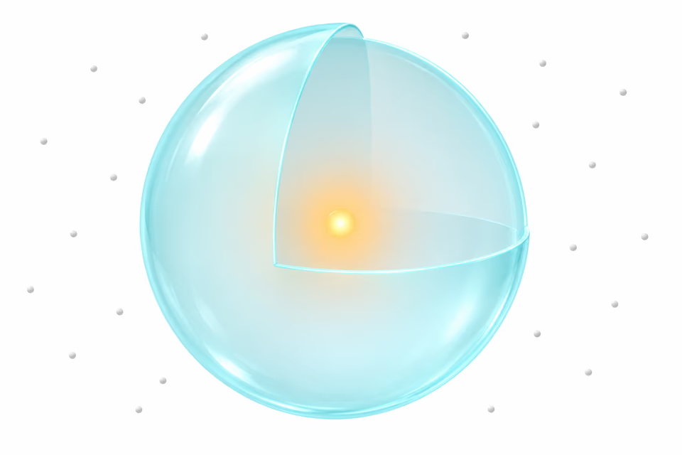
The times are readings on the camera clock. The pulse occurred at an unknown reading \(t_{0}\). These data were constructed for the problem. The extra digits let you test a prediction.
| Camera reading \(t\) (ms) | Shock radius \(R\) (m) |
|---|---|
| 0.60 | 1.5157 |
| 1.00 | 2.0000 |
| 1.80 | Reveal radius2.6390 |
Take the energy as constant. The source size and pulse duration are negligible on the observed scales. Initially neglect ambient pressure, gravity, viscosity and energy loss. A separate gas dynamics calculation gives the dimensionless multiplier \(\beta = 1.10\) in the radius law.
Your turn. Find the radius law, date the pulse and use the first two frames to predict the third radius. How much energy did the pulse deposit? Decide whether a 1% error in radius matters, and whether an ambient pressure of \(1.0 \times 10^{5}\,\text{P}\text{a}\) can still be neglected at the last frame.
Open hint 1
For the radius. The combination \(E/\rho\) contains no mass dimension. What are its remaining dimensions? How could elapsed time turn it into a length?
Open hint 2
For the missing instant. Once you have a power law, choose a power of the radius that grows linearly with time. Where should that line cross the time axis?
Read the worked solution
The clock the shock obeys
The gas has no way to tell when the camera was switched on. The time that can enter a growth law is the age of the shock, \(\tau = t - t_{0}\). In this model \(E/\rho\) has dimensions \(L^{5}T^{- 2}\). Multiplying by \(\tau^{2}\) leaves the fifth power of a length. For fixed gas properties, the only possible radius law is
There is a physical reason for that fifth power. A sphere of radius \(R\) has swept up a mass of order \(\rho R^{3}\), and the characteristic speed is of order \(R/\tau\). In a strong shock the thermal and kinetic energies have the same scaling. A mass times a speed squared then gives \(E \sim \rho R^{5}/\tau^{2}\). This argument explains the powers but leaves the multiplier undetermined.
Predict the third frame
Raise the radius to the power \(5/2\). In these coordinates the camera’s offset has a simple geometrical meaning.
For the first two frames, \(Y\) is \(2.82835\) and \(5.65685\,\text{m}^{5/2}\). Their slope is \(S \approx 7.071\,\text{m}^{5/2}\,{\text{m}\text{s}}^{- 1}\). Run the line backwards from the first point. It meets the time axis at \(t_{0} = 0.60\,\text{m}\text{s} - Y_{1}/S \approx 0.20\,\text{m}\text{s}\).
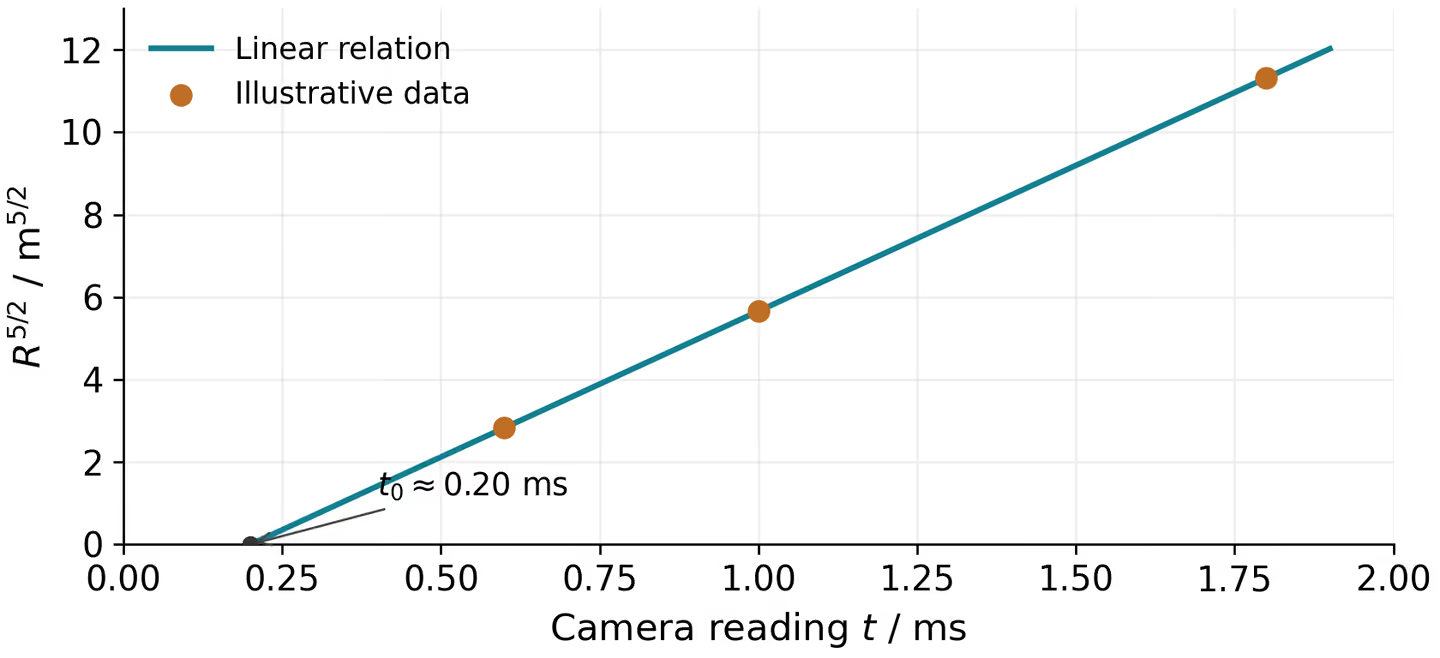
At \(1.80\,\text{m}\text{s}\) the shock is \(1.60\,\text{m}\text{s}\) old, twice its age in the middle frame. The predicted radius is \(2.0000 \times 2^{2/5} \approx 2.6390\,\text{m}\). Now uncover the third entry. We used two points to draw the line. The third had a chance to disagree.
Reading the energy from the slope
Change every timestamp by the same amount and the line slides sideways. Its slope survives. That is why the photographs give the same energy whichever clock zero the camera happened to use. A clock that runs at the wrong rate would change the slope.
There is also a way to recover the time without plotting anything. The ratio of the first two radii gives \(\tau_{2}/\tau_{1} = \left( R_{2}/R_{1} \right)^{5/2} \approx 2\). Their ages differ by \(0.40\,\text{m}\text{s}\), so the first frame caught the front at age \(0.40\,\text{m}\text{s}\). The onset falls \(0.40\,\text{m}\text{s}\) before the first reading of \(0.60\,\text{m}\text{s}\). Both the unknown energy and the multiplier have cancelled.
In seconds, \(S \approx 7.071 \times 10^{3}\,\text{m}^{5/2}\,\text{s}^{- 1}\). Either expression gives \(E \approx 3.7 \times 10^{7}\,\text{J}\). The middle frame provides a direct check with \(R = 2.00\,\text{m}\) and \(\tau = 8.0 \times 10^{- 4}\,\text{s}\). Setting the seemingly modest factor \(\beta\) equal to one would raise the estimate by the factor \({1.10}^{5} \approx 1.61\).
Which slope is a speed? Differentiating the radius gives \(v = 2R/(5\tau)\), or \(1.0 \times 10^{3}\,\text{m}\,\text{s}^{- 1}\) at the middle frame. The slope \(S\) above has units of \(\text{m}^{5/2}\,\text{s}^{- 1}\). A third possible slope, that of \(\ln\left( R/R_{*} \right)\) against \(\ln\left( \tau/\tau_{*} \right)\), is the dimensionless exponent \(2/5\). Here \(R_{*}\) and \(\tau_{*}\) are fixed reference values. Using camera time in that last plot generally bends the line.
What a radius error costs
Suppose the measured radius alone is 1% too large. The energy inferred from that frame goes up by the factor \({1.01}^{5} \approx 1.051\). A small error in finding the front can matter even when the clock is excellent. For small changes in all four inputs,
For a separate uncertainty example, take \(\rho = (1.20 \pm 0.02)\,\text{k}\text{g}\,\text{m}^{- 3}\), \(R = (2.00 \pm 0.02)\,\text{m}\), \(\beta = 1.10 \pm 0.02\) and \(\tau = (0.80 \pm 0.01)\,\text{m}\text{s}\). The four contributions to the fractional uncertainty are about 1.7%, 5.0%, 9.1% and 2.5%. Here the calibration of \(\beta\) matters most.
If those are error bounds, adding the magnitudes gives a first-order bound of about 18%. If they are independent standard uncertainties, take the square root of the sum of their squares. The result is about 11%, giving \(E = (3.7 \pm 0.4) \times 10^{7}\,\text{J}\). When a radius and the onset time come from the same fit, their errors can be correlated. The independent calculation then needs a covariance term.
Where the model starts to give way
The straight line fitted the constructed data almost perfectly. That alone tells us little about the air. An expanding sphere must displace gas against the ambient pressure \(p_{0}\). Compare the associated work scale with the deposited energy.
At the middle frame this ratio is about \(0.090\). At the last frame it is about \(0.21\). The growing volume makes the pressure check worse as the shock expands. Ambient pressure still gives a smaller energy scale than the pulse, but the last frame offers little basis for a high-precision pressure-free estimate. Turning this comparison into a numerical correction would require a model that includes ambient pressure.
Change the source
Keep the same gas, but leave the source switched on at constant power \(P\). Before doing the algebra, decide which front should grow faster as a power of time. The swept-up gas now shares an energy that grows in proportion to \(\tau\). The combination \(P\tau^{3}/\rho\) has dimensions \(L^{5}\), giving
The exponent rises from \(2/5\) to \(3/5\). The dimensionless multiplier can change when the source changes. There is also a comparison for which it cancels exactly. Take two short pulses in the same gas, in the same regime, observed at the same age. If the second front is 20% larger, the second pulse had \({1.20}^{5} \approx 2.49\) times the energy.
One for the discussion. Suppose the timestamps are reliable but the camera’s length scale is wrong by an unknown constant factor. Which of your two conclusions can another solver still check from the pictures alone? Is it the onset time, the energy, or both? Give a geometrical argument using the line you fitted.
Try a related problem
Can a sequence of orbital periods reveal how a star is losing energy?